
nflfastR
Ben Baldwin and Sebastian Carl released nflfastR yesterday to provide faster scraping of NFL play-by-play data as well as data all the way back to 2000! This builds upon the work of the nflscrapR team who paved the way for this data for NFL games between 2009 and 2019.
INTRODUCING: @nflfastR, an R package for scraping NFL data faster ⚡
— Ben Baldwin (@benbbaldwin) April 27, 2020
🏈 Play-by-play of all NFL games going back to 2000
🏈 Includes Completion Probability and CPOE going back to 2006
🏈 Fast functions for scraping team rosters and highlight videoshttps://t.co/sgrq8GdoWJ pic.twitter.com/fqbyE1pPHE
More data
With more data comes excitement - we can do new analysis with very similar code!
However, the 2000-2019 data consists of ~2.25 GB of data, 291 variables and 903,998 rows… this is 263,063,418 observations! While this is not anywhere close to too much for R to handle, it can start to feel a little intimidating to read it all into memory. I’ll be covering some tooling to work with relatively larger datasets using the same dplyr tools you know and love!
Read in the data
Ben and Sebastian were kind enough to provide all of the .RDS files for every year between 2000-2019 on GitHub for ease of download. With a quick purrr call we can download all 20 years of data and pull them into memory. We can also save them to local storage for offline access or to at least not need to re-download them down the line.
However, as mentioned before this is ~ 2 GB of data in memory, which can take a while to download and/or read in especially if you do this multiple times as opposed to in just one session. Also - there are VERY few times where you actually need to pull in all of the specific columns and/or rows for your analysis, why waste time reading in data that you don’t need?
Enter SQL
No no, I’m not going to make you learn SQL to work with this dataset, but we are going to use SQL inside R. Specifically, we’re going to play around with SQLite - in their own words:
SQLite is a C-language library that implements a small, fast, self-contained, high-reliability, full-featured, SQL database engine. SQLite is the most used database engine in the world.
What this provides for us is a super lightweight storage and query format that works nicely with R and dplyr. We don’t have to mess around with creating an entire database but rather have a small self-contained file that allows for many of the same SQL-features.
For a deeper dive on the RSQLite package, with basic and advanced usage check out the packagedown site. Additionally, the Data Carpentry guide is pretty similar to this guide but aimed at scientists.
Create the SQLite database
# <SQLiteConnection>
#   Path: /Users/thomasmock/nflscrapR/data/pbp_db.sqlite
#   Extensions: TRUE
# Write the in-memory data into the database as a table
DBI::dbWriteTable(mydb, "pbp_raw_2000-2019", raw_pbp)
# list the table
DBI::dbListTables(mydb)# [1] "pbp_raw_2000-2019"Ok - so to recap in about 2 lines of code we have created and populated a SQLite database solely through R. Now, the SQLite file is only around 1 GB compared to our 2 GB .RDS - so it’s more efficiently stored and allows us to do some other cool things as seen below.
dbplyr
Now the magic really happens: dplyr has a built-in package called dbplyr, this is a translation engine that lets you write dplyr code that is evaluated as SQL.
Full details at the dbplyr site.
The basic concept is:
Connect to a datasource/database
Query the database INSIDE the database or on disk
Pull the data into memory only when you’re ready
Open a connection
We can open the connection by calling tbl() on the database we have open (mydb) and indicating which table we want to query.
# Source:   table<pbp_raw_2000-2019> [?? x 291]
# Database: sqlite 3.30.1
# [/Users/thomasmock/nflscrapR/data/pbp_db.sqlite]

#   play_id game_id home_team away_team posteam posteam_type defteam side_of_field yardline_100
#      <dbl>   <dbl> <chr>     <chr>     <chr>   <chr>        <chr>   <chr>                <dbl>
#  1      34  2.00e9 NYG       ARI       NYG     home         ARI     NYG                     70
#  2      70  2.00e9 NYG       ARI       ARI     away         NYG     NYG                     25
#  3     106  2.00e9 NYG       ARI       ARI     away         NYG     ARI                     65
#  4     131  2.00e9 NYG       ARI       ARI     away         NYG     ARI                     63
#  5     148  2.00e9 NYG       ARI       ARI     away         NYG     ARI                     63
#  6     165  2.00e9 NYG       ARI       ARI     away         NYG     ARI                     63
#  7     190  2.00e9 NYG       ARI       NYG     home         ARI     NYG                     78
#  8     211  2.00e9 NYG       ARI       NYG     home         ARI     NYG                     70
#  9     232  2.00e9 NYG       ARI       NYG     home         ARI     NYG                     67
# 10     253  2.00e9 NYG       ARI       NYG     home         ARI     NYG                     68
# # … with more rows, and 282 more variables: game_date <dbl>, quarter_seconds_remaining <dbl>,
# #   half_seconds_remaining <dbl>, game_seconds_remaining <dbl>, game_half <chr>,
# #   quarter_end <dbl>, drive <dbl>, sp <dbl>, qtr <dbl>, down <chr>, goal_to_go <dbl>,
# #   time <chr>, yrdln <chr>, ydstogo <dbl>, ydsnet <dbl>, desc <chr>, play_type <chr>,
# #   yards_gained <dbl>, shotgun <dbl>, no_huddle <dbl>, qb_dropback <dbl>, qb_kneel <dbl>,
# #   qb_spike <dbl>, qb_scramble <dbl>, pass_length <chr>, pass_location <chr>,
# #   air_yards <dbl>, yards_after_catch <dbl>, run_location <chr>, run_gap <chr>,
# #   field_goal_result <chr>, kick_distance <dbl>, extra_point_result <chr>,
# #   two_point_conv_result <chr>, home_timeouts_remaining <dbl>,
# #   away_timeouts_remaining <dbl>, timeout <dbl>, timeout_team <chr>, td_team <chr>,
# #   posteam_timeouts_remaining <dbl>, defteam_timeouts_remaining <dbl>,
# #   total_home_score <dbl>, total_away_score <dbl>, posteam_score <dbl>, defteam_score <dbl>,
# #   score_differential <dbl>, posteam_score_post <dbl>, defteam_score_post <dbl>,
# #   score_differential_post <dbl>, no_score_prob <dbl>, opp_fg_prob <dbl>,
# #   opp_safety_prob <dbl>, opp_td_prob <dbl>, fg_prob <dbl>, safety_prob <dbl>,
# #   td_prob <dbl>, extra_point_prob <dbl>, two_point_conversion_prob <dbl>, ep <dbl>,
# #   epa <dbl>, total_home_epa <dbl>, total_away_epa <dbl>, total_home_rush_epa <dbl>,
# #   total_away_rush_epa <dbl>, total_home_pass_epa <dbl>, total_away_pass_epa <dbl>,
# #   air_epa <dbl>, yac_epa <dbl>, comp_air_epa <dbl>, comp_yac_epa <dbl>,
# #   total_home_comp_air_epa <dbl>, total_away_comp_air_epa <dbl>,
# #   total_home_comp_yac_epa <dbl>, total_away_comp_yac_epa <dbl>,
# #   total_home_raw_air_epa <dbl>, total_away_raw_air_epa <dbl>, total_home_raw_yac_epa <dbl>,
# #   total_away_raw_yac_epa <dbl>, wp <dbl>, def_wp <dbl>, home_wp <dbl>, away_wp <dbl>,
# #   wpa <dbl>, home_wp_post <dbl>, away_wp_post <dbl>, total_home_rush_wpa <dbl>,
# #   total_away_rush_wpa <dbl>, total_home_pass_wpa <dbl>, total_away_pass_wpa <dbl>,
# #   air_wpa <dbl>, yac_wpa <dbl>, comp_air_wpa <dbl>, comp_yac_wpa <dbl>,
# #   total_home_comp_air_wpa <dbl>, total_away_comp_air_wpa <dbl>,
# #   total_home_comp_yac_wpa <dbl>, total_away_comp_yac_wpa <dbl>,
# #   total_home_raw_air_wpa <dbl>, total_away_raw_air_wpa <dbl>, total_home_raw_yac_wpa <dbl>,
# #   …
Boom - 1 line of code and we now have a connection - also notice that the output has the following info at the top: > table<pbp_raw_2000-2019> [?? x 291]
Notice that it has the right number of columns (291) but an unknown number of rows. This is because the data hasn’t been read into memory yet, and it has only returned the essentially the head() of the data. We don’t pull the data into memory until we call a new function - collect() this then pulls the data as it is at that point in the pipe into memory.
Query the database
Now let’s do a basic query - we’ll time it to see how long this takes on all 263 million observations.
# Source:   lazy query [?? x 4]
# Database: sqlite 3.30.1 [/Users/thomasmock/nflscrapR/data/pbp_db.sqlite]
# Groups:   season
#    season play_type avg_yds     n
#     <dbl> <chr>       <dbl> <int>
#  1   2000 pass         5.84 17567
#  2   2000 run          4.08 13682
#  3   2001 pass         5.85 17264
#  4   2001 run          4.04 13500
#  5   2002 pass         5.85 18313
#  6   2002 run          4.27 13746
#  7   2003 pass         5.79 17322
#  8   2003 run          4.24 14033
#  9   2004 pass         6.12 17238
# 10   2004 run          4.24 13828

# 1.048 sec elapsed
So we used our traditional dplyr code, it ran as SQL on the backend and took about 1 sec. Now, 1 sec is not THAT fast - and the same operation IN memory would be about 0.2 sec, but we save a lot of time on the read and can do lots of ad-hoc queries without pulling the data in. Also imagine a world where the data is much larger than memory, this same workflow would work on 100 GB of data or even petabytes of data with translation to spark via sparklyr for example.
Collect the data
Lastly - we can also pull the data into memory, via collect(). This allows us to take the data and either continue to work with the summary or pass it to something like ggplot2.
tic()
pbp_db %>%
  select(play_type, yards_gained, penalty, season) %>%
  filter(play_type %in% c("run", "pass"), penalty == 0) %>%
  group_by(season, play_type) %>%
  summarize(avg_yds = mean(yards_gained, na.rm = TRUE),
            n = n()) %>%
  collect() %>%
  ggplot(aes(x = season, y = avg_yds, color = play_type)) +
  geom_line()
toc()
# 1.451 sec elapsed 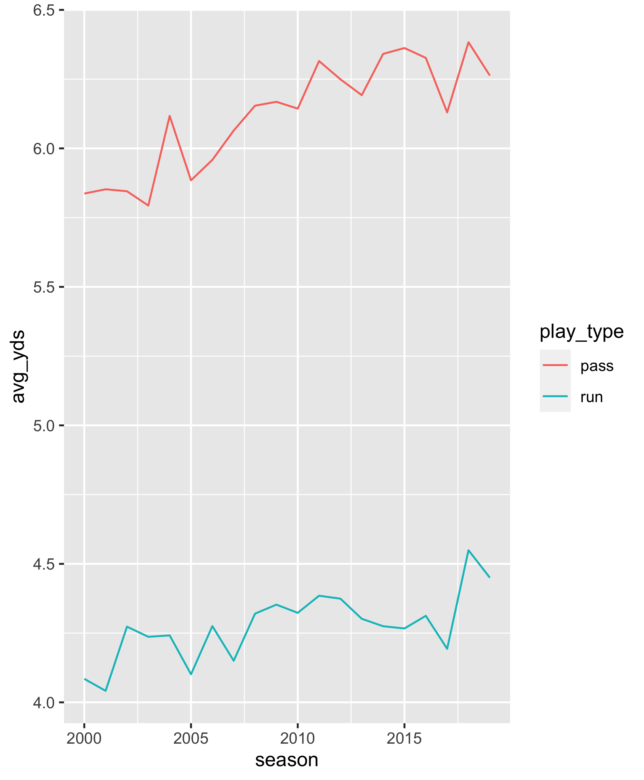
So, in about 1.5 seconds we we’re able to query all of 2000-2019 and get a very basic ggplot. Cool!
TLDR
Altogether now skipping the additional info. You can see just how succintly you can use this method. It’s just like reading in other data formats!
library(dplyr)

pbp_db <- dplyr::tbl(DBI::dbConnect(RSQLite::SQLite(), "data/pbp_db.sqlite"), "pbp_raw_2000-2019")

pbp_db %>%
  select(play_type, yards_gained, penalty, season) %>%
  filter(play_type %in% c("run", "pass"), penalty == 0) %>%
  group_by(season, play_type) %>%
  summarize(avg_yds = mean(yards_gained, na.rm = TRUE),
            n = n()) %>%
  collect()
# A tibble: 40 x 4
# Groups: season [20]
# season play_type avg_yds n
# <dbl> <chr> <dbl> <int>
# 1 2000 pass 5.84 17567
# 2 2000 run 4.08 13682
# 3 2001 pass 5.85 17264
# 4 2001 run 4.04 13500
# 5 2002 pass 5.85 18313
# 6 2002 run 4.27 13746
# 7 2003 pass 5.79 17322
# 8 2003 run 4.24 14033
# 9 2004 pass 6.12 17238
# 10 2004 run 4.24 13828
# … with 30 more rowsAdditional Notes
I would be remiss to not mention alternative methods to getting relatively normal-sized data into memory. Using R is a great experience for small to medium sized datasets.
-
data.table::fread()is super fast for reading in files-
data.tableis also extremely fast when operating on in-memory data - Just like with
dplyranddbplyrfor reading from databases,dtplyrlets you usedplyrcall to rundata.tablequeries – I’ll cover this in a follow-up post
-
-
vroom::vroom()is even faster for reading in data in some situations
In this case for our toy examples, pure dplyr, data.table and dtplyr are all essentially the same speed, about 0.1 - 0.2 seconds to run the same summary in-memory compared to ~ 1 sec via SQLite. However, the time-savings here are very much on read-in.
data.table::fread() takes about 28 seconds to read in the full csv, vroom::vroom() takes about 20 seconds to read in the full csv, and then either data.table or dplyr take between 0.1 - 0.2 seconds to perform the aggregation. This is compared to the ~ 1 second to aggregate with the same analysis via dbplyr + RSQLite.
tic()

dt_pbp <- fread("pbp_large.csv")

toc()
# |--------------------------------------------------|
# |==================================================|
# |--------------------------------------------------|
# |==================================================|
# 27.875 sec elapsedThe last thing I’ll add is that if you want to do additional modeling or work with the entire dataset over a long period of time, I think it makes sense to read it into memory to get the speed improvements of in-memory computation and access to the full range of R’s capability. Just wanted to bring up that it’s possible to rapidly work on relatively large datasets and only pull into memory when you are ready.
─ Session info ───────────────────────────────────────────────────────────────
 setting  value
 version  R version 4.2.0 (2022-04-22)
 os       macOS Monterey 12.2.1
 system   aarch64, darwin20
 ui       X11
 language (EN)
 collate  en_US.UTF-8
 ctype    en_US.UTF-8
 tz       America/Chicago
 date     2022-04-28
 pandoc   2.18 @ /Applications/RStudio.app/Contents/MacOS/quarto/bin/tools/ (via rmarkdown)
 quarto   0.9.294 @ /usr/local/bin/quarto

─ Packages ───────────────────────────────────────────────────────────────────
 package     * version    date (UTC) lib source
 DBI         * 1.1.2      2021-12-20 [1] CRAN (R 4.2.0)
 dplyr       * 1.0.8      2022-02-08 [1] CRAN (R 4.2.0)
 dtplyr      * 1.2.1      2022-01-19 [1] CRAN (R 4.2.0)
 forcats     * 0.5.1      2021-01-27 [1] CRAN (R 4.2.0)
 ggplot2     * 3.3.5      2021-06-25 [1] CRAN (R 4.2.0)
 nflfastR    * 4.3.0.9009 2022-04-26 [1] Github (nflverse/nflfastR@8afc872)
 pryr        * 0.1.5      2021-07-26 [1] CRAN (R 4.2.0)
 purrr       * 0.3.4      2020-04-17 [1] CRAN (R 4.2.0)
 readr       * 2.1.2      2022-01-30 [1] CRAN (R 4.2.0)
 RSQLite     * 2.2.12     2022-04-02 [1] CRAN (R 4.2.0)
 sessioninfo * 1.2.2      2021-12-06 [1] CRAN (R 4.2.0)
 stringr     * 1.4.0      2019-02-10 [1] CRAN (R 4.2.0)
 tibble      * 3.1.6      2021-11-07 [1] CRAN (R 4.2.0)
 tictoc      * 1.0.1      2021-04-19 [1] CRAN (R 4.2.0)
 tidyr       * 1.2.0      2022-02-01 [1] CRAN (R 4.2.0)
 tidyverse   * 1.3.1      2021-04-15 [1] CRAN (R 4.2.0)

 [1] /Library/Frameworks/R.framework/Versions/4.2-arm64/Resources/library

──────────────────────────────────────────────────────────────────────────────