reactable - An Interactive Tables Guide

Part 2: How to draw the rest of the owl.

NFL
tidyverse
tables
Author

Thomas Mock

Published

May 15, 2020

A charcoal drawing of an owl with two steps

It is a beautiful owl/table though isn’t it?


Part 2 of this guide will go through how to in fact draw the rest of the owl, as the previous post barely covered the how and instead focused on a clean final product.

reactable - interactive data tables

reactable is an R wrapper for the react table javascript library. Greg Lin at RStudio recently made this package and you can install it from CRAN with install.packages("reactable"). I adapted this table from some examples at the reactable package site.

If you want to go much deeper than this basic guide, check out the reactable site, which has lots of examples!

Raw data comes from: Pro Football Reference & Over the Cap

Read in the Data

I’ve gone through collecting the data and have put into a non-tidy wide format for Salary Rank, playoff week and appearances, Total appearances, and finally salary from 2014-2019. The raw CSV is available on GitHub

library(reactable) # for interactive tables
library(tidyverse) # all the things
── Attaching packages ─────────────────────────────────────── tidyverse 1.3.1 ──
✔ ggplot2 3.3.5     ✔ purrr   0.3.4
✔ tibble  3.1.6     ✔ dplyr   1.0.8
✔ tidyr   1.2.0     ✔ stringr 1.4.0
✔ readr   2.1.2     ✔ forcats 0.5.1
── Conflicts ────────────────────────────────────────── tidyverse_conflicts() ──
✖ dplyr::filter() masks stats::filter()
✖ dplyr::lag()    masks stats::lag()
library(htmltools) # for building div/links
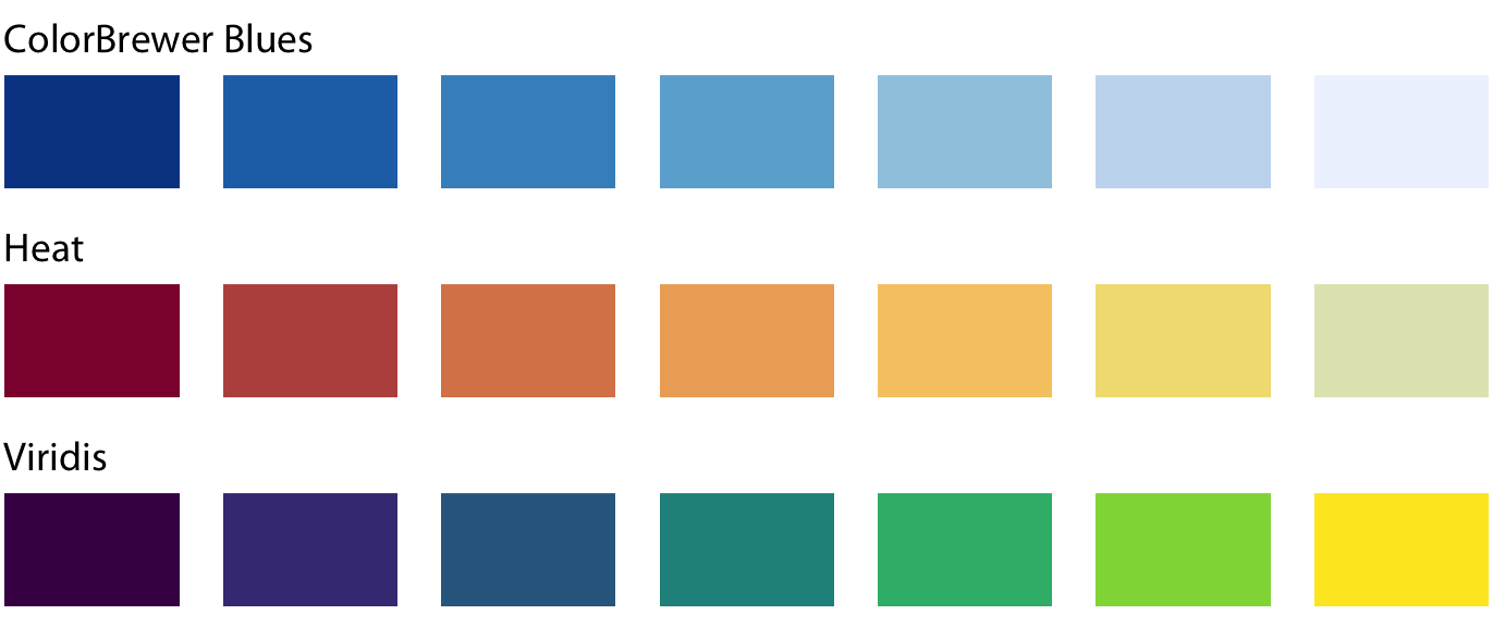
library(paletteer) # for all the palettes

playoff_salary <- read_csv("playoff_salary.csv")
Rows: 36 Columns: 8
── Column specification ────────────────────────────────────────────────────────
Delimiter: ","
chr (1): player
dbl (7): Salary Rank, Wildcard, Division, Conference, Superbowl, Total, salary

ℹ Use `spec()` to retrieve the full column specification for this data.
ℹ Specify the column types or set `show_col_types = FALSE` to quiet this message.
glimpse(playoff_salary)
Rows: 36
Columns: 8
$ `Salary Rank` <dbl> 1, 2, 3, 4, 5, 6, 7, 8, 9, 10, 11, 12, 13, 14, 15, 16, 1…
$ player        <chr> "Matt Stafford", "Ben Roethlisberger", "Aaron Rodgers", …
$ Wildcard      <dbl> 2, 3, 2, 2, 1, 1, 1, 1, 2, 1, 2, 2, 4, 1, 2, 0, 0, 1, 1,…
$ Division      <dbl> 0, 3, 4, 2, 0, 2, 1, 1, 2, 5, 1, 2, 4, 0, 2, 1, 1, 1, 1,…
$ Conference    <dbl> 0, 1, 3, 1, 0, 1, 0, 0, 1, 5, 0, 0, 1, 0, 1, 1, 1, 1, 0,…
$ Superbowl     <dbl> 0, 0, 0, 0, 0, 1, 0, 0, 1, 4, 0, 0, 1, 0, 0, 0, 1, 0, 0,…
$ Total         <dbl> 2, 7, 9, 5, 1, 5, 2, 2, 6, 15, 3, 4, 10, 1, 5, 2, 3, 3, …
$ salary        <dbl> 129.7, 127.7, 125.6, 125.2, 124.2, 118.0, 117.3, 106.1, …

Basics of reactable

A very basic reactable table can be created as so:

playoff_salary %>%
  reactable()

Immediately we have reactive table split into 4x pages with 10 observations per page.

The core parts we want to change are:
- Conditional color formatting for Total Appearances and Salary
- All on one page
- Change the font

Conditional Colors

Like most things in R there are MANY ways to generate indeterminate length color palettes. For more info about using color to represent data values check out Claus Wilke’s book section. Importantly - we want a sequential/continuous color scale.

Per Claus:

Such a scale contains a sequence of colors that clearly indicate (i) which values are larger or smaller than which other ones and (ii) how distant two specific values are from each other. The second point implies that the color scale needs to be perceived to vary uniformly across its entire range.

Sequential scales can be based on a single hue (e.g., from dark blue to light blue) or on multiple hues (e.g., from dark red to light yellow) (Figure 4.3). Multi-hue scales tend to follow color gradients that can be seen in the natural world, such as dark red, green, or blue to light yellow, or dark purple to light green. The reverse, e.g. dark yellow to light blue, looks unnatural and doesn’t make a useful sequential scale.

Figure 4.3

Now there are plenty of palettes to choose from, such as viridis, RColorBrewer, ggthemes, as well as a nice meta collection via paletteer!

Now it’s often hard to keep track of these palettes and what they actually look like.

To display ANY palette or vector of colors in R you can use scales::show_col() - scales comes along with ggplot2 & the tidyverse, so you probably don’t need to install it (just load it)! Reference: StackOverflow and scales.


Attaching package: 'scales'
The following object is masked from 'package:purrr':

    discard
The following object is masked from 'package:readr':

    col_factor
scales::show_col(c("red", "black", "blue", "purple"))

scales::show_col() also works with palettes/vectors.

scales::show_col() also works with paletteer or really any other palette package to display palettes/vectors. You just need to supply > 1 color as a character vector and you’re good to go!

Now that we understand how to show colors, I’ll explain a bit more about our coloring function.

Color Function

I borrowed my function to generate colors scales through grDevices::colorRamp() from Greg Lin’s examples. This makes use of colorRamp to generate a sequence of colors and then pull them according to a sliding scale normalized to 0-1.

# greg's palette
scales::show_col(c("#ffffff", "#f2fbd2", "#c9ecb4", "#93d3ab", "#35b0ab"))

Back to our color scale, we can display an example step-by-step.

# Function by Greg Lin
# Notice bias here = a positive number. 
# Higher values give more widely spaced colors at the high end

make_color_pal <- function(colors, bias = 1) {
  get_color <- colorRamp(colors, bias = bias)
  function(x) rgb(get_color(x), maxColorValue = 255)
}

good_color <- make_color_pal(c("#ffffff", "#f2fbd2", "#c9ecb4", "#93d3ab", "#35b0ab"), bias = 2)

# Generate a vector of example numbers between 0 and 1
seq(0.1, 0.9, length.out = 12)
 [1] 0.1000000 0.1727273 0.2454545 0.3181818 0.3909091 0.4636364 0.5363636
 [8] 0.6090909 0.6818182 0.7545455 0.8272727 0.9000000
# create matching colors
good_color(seq(0.1, 0.9, length.out = 12))
 [1] "#E9F8CB" "#D9F2C0" "#C9ECB4" "#BDE6B2" "#B0E0AF" "#A4DAAD" "#97D5AB"
 [8] "#88CFAB" "#79C9AB" "#69C3AB" "#5ABDAB" "#4AB8AB"
# display the colors
seq(0.1, 0.9, length.out = 12) %>% 
  good_color() %>% 
  scales::show_col()

Format by value

reactable has a section on conditional styling - either logical or based on a continuous scale. You can use R or JavaScript functions to change the style of cells.

The core table is seen below with comments added to highlight some emphasized changes.

playoff_salary %>% 
  mutate(salary = round(salary, 1)) %>% 
    
    ##########################
    ### This section changed
    ##########################
  reactable(
    # ALL one page option (no scrolling or page swapping)
    pagination = TRUE,
    # compact for an overall smaller table width wise
    compact = TRUE,
    # borderless - TRUE or FALSE
    borderless = FALSE,
    # Stripes - TRUE or FALSE
    striped = FALSE,
    # fullWidth - either fit to width or not
    fullWidth = FALSE,
    # apply defaults
    # 100 px and align to center of column
    defaultColDef = colDef(
      align = "center",
      minWidth = 100
    ))

To actually change the color according to our color scale, we can use the below code. We are defining an anonymous (unsaved) function and using our good_color() function to generate values along our scale.

playoff_salary %>% 
  mutate(salary = round(salary, 1)) %>% 
  reactable(
    # ALL one page (no scrolling or page swapping)
    pagination = TRUE,
    # compact for an overall smaller table width wise
    compact = TRUE,
    # borderless - TRUE or FALSE
    borderless = FALSE,
    # Stripes - TRUE or FALSE
    striped = FALSE,
    # fullWidth - either fit to width or not
    fullWidth = FALSE,
    # apply defaults
    # 100 px and align to center of column
    defaultColDef = colDef(
      align = "center",
      minWidth = 100
    ),
    
      ##########################
      ### This section changed
      ##########################
    
    # This part allows us to apply specific things to each column
    columns = list(
      salary = colDef(
        name = "Salary",
        style = function(value) {
          value
          normalized <- (value - min(playoff_salary$salary)) / (max(playoff_salary$salary) - min(playoff_salary$salary))
          color <- good_color(normalized)
          list(background = color)
        }
      )
      )
    )

Woo! We now have a color scale ranging from about 4 million to 130 million, but let’s indicate Millions with an M so that people don’t get confused. There is a bit of JavaScript code here - please note, I don’t know JavaScript BUT JavaScript can be a functional programming language, so I bet the code below looks readable to you! In this case, cellInfo.value is like dataframe$value, so it will parse through and apply the function to each cell in our table.

I adapted this code from StackOverflow.

"function(cellInfo) { return '$' + cellInfo.value + ' M'}"

Formatting numbers all together now, with both the color function and the JS function to add dollar + M to our cells.

playoff_salary %>% 
  mutate(salary = round(salary, 1)) %>% 
  reactable(
    # ALL one page (no scrolling or page swapping)
    pagination = TRUE,
    # compact for an overall smaller table width wise
    compact = TRUE,
    # borderless - TRUE or FALSE
    borderless = FALSE,
    # Stripes - TRUE or FALSE
    striped = FALSE,
    # fullWidth - either fit to width or not
    fullWidth = FALSE,
    # apply defaults
    # 100 px and align to center of column
    defaultColDef = colDef(
      align = "center",
      minWidth = 100
    ),
    
      ##########################
      ### This section changed
      ##########################
    
    # This part allows us to apply specific things to each column
    columns = list(
      salary = colDef(
        # note I can re-define the name of salary to Salary
        name = "Salary",
        style = function(value) {
          value
          # normalize each value relative to min/max (scale between 0 and 1)
          normalized <- (value - min(playoff_salary$salary)) / (max(playoff_salary$salary) - min(playoff_salary$salary))
          # assign a color base on the normalized value
          color <- good_color(normalized)
          # return a list object of the color
          list(background = color)
        },
        # This is javascript to take the cell's value and add an M to the value
        # Note that because this is done at the JS level
        # the columns still sort properly (they're still numbers!)
        # There are built in format currency options, but not one
        # for compressing to Millions AND to dollars for example
        cell = JS("function(cellInfo) { return '$' + cellInfo.value + ' M'}")
      )
      )
  )

Format Total Column

Now we can use a similar approach to add color to our Total playoff appearances column.

tbl <- playoff_salary %>% 
  mutate(salary = round(salary, 1)) %>% 
  reactable(
    pagination = FALSE,
    compact = TRUE,
    borderless = FALSE,
    striped = FALSE,
    fullWidth = FALSE,
    defaultColDef = colDef(
      align = "center",
      minWidth = 100
    ),
    # Add theme for the top border
    theme = reactableTheme(
      headerStyle = list(
        "&:hover[aria-sort]" = list(background = "hsl(0, 0%, 96%)"),
        "&[aria-sort='ascending'], &[aria-sort='descending']" = list(background = "hsl(0, 0%, 96%)"),
        borderColor = "#555"
      )
    ),
    columns = list(
      salary = colDef(
        name = "Salary",
        style = function(value) {
          value
          normalized <- (value - min(playoff_salary$salary)) / (max(playoff_salary$salary) - min(playoff_salary$salary))
          color <- good_color(normalized)
          list(background = color)
        },
        cell = JS("function(cellInfo) {return '$' + cellInfo.value + 'M'}")
      ),
      
      ##########################
      ### This section changed
      ##########################
      # We can now do a similar function for Total to color according to a
      # normalized scale
      Total = colDef(
        style = function(value) {
          value
          normalized <- (value - min(playoff_salary$Total)) / (max(playoff_salary$Total) - min(playoff_salary$Total))
          color <- good_color(normalized)
          list(background = color)
        },
        # we'll also add a border to the left of this column
        class = "border-left"
      ),
      # and change the width/alignment of the player column
      player = colDef(
        # Change player to Name
        name = "Name",
        # Widen it so that player names don't get wrapped as much
        minWidth = 140,
        # Align left as it is a wide column
        # this overrides the default above
        align = "left"
      )
    )
  )

tbl

CSS & Fonts

Note that the above table is essentially done. It has all the core changes we wanted (conditional color and interactivity). Everything below is extra1 stuff that I am also adapting from Greg’s example with the Women’s World Cup table.

  • 1 Extra can be good! It’s just sometimes hard… see RMarkdown Book for more

  • Build structure

    By building up our plot inside div containers and assiging a class we can use CSS to further style or add to our table. The main things I’m interested in is changing the base font to one I love (Fira Mono)! However, Greg included some niceties for some additional table formatting that I copied over as well.

    My mental model of div building is that it’s like nesting dolls. Main div which is the whole table, header and footer, and then additional nested div for other classes that we can call against. :::{.column-page}

    div(
      # this class can be called with CSS now via .salary
      class = "salary",
      div(
        # this can be called with CSS now via .title
        class = "title",
        h2("2014-2019 Salary and Playoff Appearances"),
        # This is kind of like a sub-title, but really it's just raw text
        "QBs limited to playoff games where they threw a pass"
      ),
      # The actual table
      tbl,
      # I use a span here so I can assigna  color to this text
      tags$span(style = "color:#C8C8C8", "TABLE: @THOMAS_MOCK | DATA: PRO-FOOTBALL-REFERENCE.COM & OVERTHECAP.COM")
    )

    2014-2019 Salary and Playoff Appearances

    QBs limited to playoff games where they threw a pass
    TABLE: @THOMAS_MOCK | DATA: PRO-FOOTBALL-REFERENCE.COM & OVERTHECAP.COM

    :::

    Import Google Font

    I want to use a Google font (Karla + Fira Mono).

    You can see all the Google Fonts here. At fonts.google.com you’ll:
    - Search for specific fonts
    - Select the Style you want (+ button)
    - Open the sidebar to extract the API call for embedding

    Example image below

    Steps to select, get and copy embed for Google Fonts

    You then paste the text inside the <link > into a tags$link() call from htmltools package.

    For example:

    <link href="https://fonts.googleapis.com/css?family=Karla:400,700|Fira+Mono&display=fallback" rel="stylesheet">

    turns into the below:

    tags$link(href = "https://fonts.googleapis.com/css?family=Karla:400,700|Fira+Mono&display=fallback", rel = "stylesheet")

    Add CSS

    This is a CSS chunk and the CSS is applied to objects matching their name, ie .salary matches the div we built earlier, .number applies to all class = number from our table, .title applies to the class = title in our table.

    Note that if I work locally not all of this will show up, but once the complete RMarkdown is knit together it will work.

    .salary {
      font-family: Karla, "Helvetica Neue", Helvetica, Arial, sans-serif;
      font-size: 14px;
    }
    
    .number {
      font-family: "Fira Mono", Consolas, Monaco, monospace;
      font-size: 16px;
      line-height: 30px;
      white-space: pre;
    }
    
    .title {
      margin: 18px 0;
      font-size: 16px;
    }
    
    .title h2 {
      font-size: 20px;
      font-weight: 600;
    }
    
    .header:hover,
    .header[aria-sort="ascending"],
    .header[aria-sort="descending"] {
      background-color: #eee;
    }
    
    .salary-table {
      margin-bottom: 20px;
    }
    
    /* Align header text to the bottom */
    .header,
    .group-header {
      display: flex;
      flex-direction: column;
      justify-content: flex-end;
    }
    
    .header {
      border-bottom-color: #555;
      font-size: 13px;
      font-weight: 400;
      text-transform: uppercase;
    }
    
    /* Highlight headers when sorting */
    .header:hover,
    .header[aria-sort="ascending"],
    .header[aria-sort="descending"] {
      background-color: #eee;
    }
    
    .border-left {
      border-left: 2px solid #555;
    }
    
    /* Use box-shadow to create row borders that appear behind vertical borders */
    .cell {
      box-shadow: inset 0 -1px 0 rgba(0, 0, 0, 0.15);
    }

    Full Code

    Below is the raw code to generate the table altogether now. This is all adapted from the reactable cookbook.

    The CSS and HTML helpers do some light-lifting for custom text and borders.

    make_color_pal <- function(colors, bias = 1) {
      get_color <- colorRamp(colors, bias = bias)
      function(x) rgb(get_color(x), maxColorValue = 255)
    }
    
    good_color <- make_color_pal(c("#ffffff", "#f2fbd2", "#c9ecb4", "#93d3ab", "#35b0ab"), bias = 2)
    
    tbl <- playoff_salary %>%
      arrange(desc(salary)) %>%
      mutate(
        `Salary Rank` = rank(desc(salary)),
        salary = round(salary, 1)
      ) %>%
      select(`Salary Rank`, player:Superbowl, everything()) %>%
      reactable(
        pagination = FALSE,
        compact = TRUE,
        borderless = FALSE,
        striped = FALSE,
        fullWidth = FALSE,
        theme = reactableTheme(
          headerStyle = list(
            "&:hover[aria-sort]" = list(background = "hsl(0, 0%, 96%)"),
            "&[aria-sort='ascending'], &[aria-sort='descending']" = list(background = "hsl(0, 0%, 96%)"),
            borderColor = "#555"
          )
        ),
        defaultColDef = colDef(
          align = "center",
          minWidth = 100
        ),
        columns = list(
          salary = colDef(
            name = "Salary",
            style = function(value) {
              value
              normalized <- (value - min(playoff_salary$salary)) / (max(playoff_salary$salary) - min(playoff_salary$salary))
              color <- good_color(normalized)
              list(background = color)
            },
            cell = JS("function(cellInfo) {
                              return cellInfo.value + 'M'}")
          ),
          Total = colDef(
            style = function(value) {
              value
              normalized <- (value - min(playoff_salary$Total)) / (max(playoff_salary$Total) - min(playoff_salary$Total))
              color <- good_color(normalized)
              list(background = color)
            },
            class = "border-left"
          ),
          player = colDef(
            name = "Name",
            minWidth = 140,
            align = "left"
          )
        )
      )


    div(
      class = "salary",
      div(
        class = "title",
        h2("2014-2019 Salary and Playoff Appearances"),
        "QBs limited to playoff games where they threw a pass"
      ),
      tbl,
      tags$span(style = "color:#C8C8C8", "TABLE: @THOMAS_MOCK | DATA: PRO-FOOTBALL-REFERENCE.COM & OVERTHECAP.COM")
    )
    tags$link(href = "https://fonts.googleapis.com/css?family=Karla:400,700|Fira+Mono&display=fallback", rel = "stylesheet")
    .salary {
      font-family: Karla, "Helvetica Neue", Helvetica, Arial, sans-serif;
      font-size: 14px;
    }
    
    .number {
      font-family: "Fira Mono", Consolas, Monaco, monospace;
      font-size: 16px;
      line-height: 30px;
      white-space: pre;
    }
    
    .title {
      margin: 18px 0;
      font-size: 16px;
    }
    
    .title h2 {
      font-size: 20px;
      font-weight: 600;
    }
    
    
    .header:hover,
    .header[aria-sort="ascending"],
    .header[aria-sort="descending"] {
      background-color: #eee;
    }
    
    .salary-table {
      margin-bottom: 20px;
    }
    
    /* Align header text to the bottom */
    .header,
    .group-header {
      display: flex;
      flex-direction: column;
      justify-content: flex-end;
    }
    
    .header {
      border-bottom-color: #555;
      font-size: 13px;
      font-weight: 400;
      text-transform: uppercase;
    }
    
    /* Highlight headers when sorting */
    .header:hover,
    .header[aria-sort="ascending"],
    .header[aria-sort="descending"] {
      background-color: #eee;
    }
    
    .border-left {
      border-left: 2px solid #555;
    }
    
    /* Use box-shadow to create row borders that appear behind vertical borders */
    .cell {
      box-shadow: inset 0 -1px 0 rgba(0, 0, 0, 0.15);
    }
    ─ Session info ───────────────────────────────────────────────────────────────
     setting  value
     version  R version 4.2.0 (2022-04-22)
     os       macOS Monterey 12.2.1
     system   aarch64, darwin20
     ui       X11
     language (EN)
     collate  en_US.UTF-8
     ctype    en_US.UTF-8
     tz       America/Chicago
     date     2022-04-28
     pandoc   2.18 @ /Applications/RStudio.app/Contents/MacOS/quarto/bin/tools/ (via rmarkdown)
     quarto   0.9.294 @ /usr/local/bin/quarto
    
    ─ Packages ───────────────────────────────────────────────────────────────────
     package     * version date (UTC) lib source
     dplyr       * 1.0.8   2022-02-08 [1] CRAN (R 4.2.0)
     forcats     * 0.5.1   2021-01-27 [1] CRAN (R 4.2.0)
     ggplot2     * 3.3.5   2021-06-25 [1] CRAN (R 4.2.0)
     htmltools   * 0.5.2   2021-08-25 [1] CRAN (R 4.2.0)
     paletteer   * 1.4.0   2021-07-20 [1] CRAN (R 4.2.0)
     purrr       * 0.3.4   2020-04-17 [1] CRAN (R 4.2.0)
     reactable   * 0.2.3   2020-10-04 [1] CRAN (R 4.2.0)
     readr       * 2.1.2   2022-01-30 [1] CRAN (R 4.2.0)
     scales      * 1.2.0   2022-04-13 [1] CRAN (R 4.2.0)
     sessioninfo * 1.2.2   2021-12-06 [1] CRAN (R 4.2.0)
     stringr     * 1.4.0   2019-02-10 [1] CRAN (R 4.2.0)
     tibble      * 3.1.6   2021-11-07 [1] CRAN (R 4.2.0)
     tidyr       * 1.2.0   2022-02-01 [1] CRAN (R 4.2.0)
     tidyverse   * 1.3.1   2021-04-15 [1] CRAN (R 4.2.0)
    
     [1] /Library/Frameworks/R.framework/Versions/4.2-arm64/Resources/library
    
    ──────────────────────────────────────────────────────────────────────────────