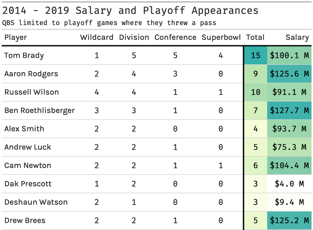
gt - a (G)rammar of (T)ables

Not to be confused with a Game of Thrones

NFL
tidyverse
tables
Author

Thomas Mock

Published

May 18, 2020

Preview of the table to come

A preview of the table to come!

gt package - a (g)rammar of (t)ables

gt is an R package for generating formatted tables from dataframes in R with a Grammar of Tables.

If you want to go deeper than this basic guide, check out the gt site, which has lots of examples!

Raw data comes from: Pro Football Reference & Over the Cap

Component parts of a gt table

Per the package website, gt has the following component parts:

The parts (roughly from top to bottom) are:

  • the Table Header (optional; with a title and possibly a subtitle)
  • the Stub and the Stub Head (optional; contains row labels, optionally within row groups having row group labels and possibly summary labels when a summary is present)
  • the Column Labels (contains column labels, optionally under spanner column labels)
  • the Table Body (contains columns and rows of cells)
  • the Table Footer (optional; possibly with footnotes and source notes)

As you can see it is fleshing out the idea of formatting or adding various parts of the table in a robust way.


Read in the Data

I’ve gone through collecting the data and have put into a non-tidy wide format for Salary Rank, playoff week and appearances, Total appearances, and finally salary from 2014-2019. The raw CSV is available on GitHub

library(gt) # for static tables
library(tidyverse) # all the things
library(paletteer) # for all the palettes

playoff_salary <- read_csv("playoff_salary.csv")
Rows: 36 Columns: 7
── Column specification ────────────────────────────────────────────────────────
Delimiter: ","
chr (1): player
dbl (6): Wildcard, Division, Conference, Superbowl, Total, salary

ℹ Use `spec()` to retrieve the full column specification for this data.
ℹ Specify the column types or set `show_col_types = FALSE` to quiet this message.
glimpse(playoff_salary)
Rows: 36
Columns: 7
$ player     <chr> "Tom Brady", "Aaron Rodgers", "Russell Wilson", "Ben Roethl…
$ Wildcard   <dbl> 1, 2, 4, 3, 2, 2, 2, 1, 2, 2, 2, 2, 1, 2, 0, 0, 1, 1, 1, 1,…
$ Division   <dbl> 5, 4, 4, 3, 2, 2, 2, 2, 1, 2, 1, 1, 2, 0, 2, 2, 0, 1, 0, 1,…
$ Conference <dbl> 5, 3, 1, 1, 0, 1, 1, 0, 0, 1, 0, 0, 1, 0, 2, 1, 0, 1, 0, 0,…
$ Superbowl  <dbl> 4, 0, 1, 0, 0, 0, 1, 0, 0, 0, 0, 0, 1, 0, 1, 1, 0, 0, 0, 0,…
$ Total      <dbl> 15, 9, 10, 7, 4, 5, 6, 3, 3, 5, 3, 3, 5, 2, 5, 4, 1, 3, 1, …
$ salary     <dbl> 100.065, 125.602, 91.114, 127.690, 93.700, 75.264, 104.374,…

Basics of gt

A very basic gt table can be created as so:

playoff_salary %>%
  head() %>%
  gt()
player Wildcard Division Conference Superbowl Total salary
Tom Brady 1 5 5 4 15 100.065
Aaron Rodgers 2 4 3 0 9 125.602
Russell Wilson 4 4 1 1 10 91.114
Ben Roethlisberger 3 3 1 0 7 127.690
Alex Smith 2 2 0 0 4 93.700
Andrew Luck 2 2 1 0 5 75.264

Immediately we have a basic table with minimal formatting.

The core parts we want to change are:
- Conditional color formatting for Total Appearances and Salary
- Change the fonts
- Add borders

Conditional Colors

We covered conditional colors in the previous post - check it out if you have further questions about building or using palettes.

A MAJOR value add that gt provides is rather than having to write our own palette parser it has a built in one via gt::data_color()! Just to refresh us on our palette, we’re using an adaptation of the viridis palette.

scales::show_col(c("#ffffff", "#f2fbd2", "#c9ecb4", "#93d3ab", "#35b0ab"))

For today’s example, we’ll use one from paletteer as well! Notice that printing paletteer::d() directly attaches the colors in the console, and to use it as a plain old character vector, we’ll need to wrap it in as.character() OR pipe it forward like palette %>% as.character().

paletteer::paletteer_d("ggsci::red_material", n = 6) %>%
  as.character() %>%
  scales::show_col()

I’d also like to introduce a function to generate colors from the scales package. scales::col_numeric() can generate continuous color scales based off a vector of colors. Notice that it operates differently than our other color function that is normalized between 0 and 1. This one takes ANY number and should be used with a vector of numbers. Notice the behavior with single colors generates the same color every time (nothing to scale against since we used domain = NULL).

red_color_generator <- scales::col_numeric(c("red", "white"), domain = NULL)

red_color_generator(50) %>% scales::show_col()

However, if you pass a vector to this, you get the expected behavior!

red_color_generator(seq(10, 60, by = 10)) %>% scales::show_col()

Alternatively, you could define domain to be part of the range of your values. This is expanded with example code below

# Define a specific range color generator
red_color_generator_ranged <- scales::col_numeric(c("red", "white"), domain = c(0, 100))

# define a few points along the range
closer_to_red <- red_color_generator_ranged(25)
between_red_white <- red_color_generator_ranged(50)
closer_to_white <- red_color_generator_ranged(75)

# combine and show colors
c(closer_to_red, between_red_white, closer_to_white) %>% scales::show_col()

You could imagine doing something like below for the domain setting. However, again note that we don’t really need to define domain for our example here. gt will pass the data column through to the data_color() function into scales::col_numeric() directly as a vector.

# Base version
my_domain <- c(min(df$col_of_interest), max(df$col_of_interest))

# OR

# tidyverse version if you wanted to try it that way
my_domain <- c(
  summarize(df, min = min(col_of_interest)) %>% pull(min),
  summarize(df, max = max(col_of_interest)) %>% pull(max)
)

red_color_generator_ranged <- scales::col_numeric(c("red", "white"),
  domain = my_domain
)

Format by value

gt has a built in function to color data cells - based on either logical or based on a continuous scale. You can use R functions or additional packages to generate indeterminate length palettes.

The core table is seen below with comments added to highlight some emphasized changes.

playoff_salary %>%
  head() %>%
  gt() %>%
  data_color(
    columns = vars(salary),
    colors = scales::col_numeric(
      # Using a function from paletteer to generate a vector of colors
      # Note that you need to wrap paletteer_d outputs in as.character()
      palette = as.character(paletteer::paletteer_d("ggsci::red_material", n = 5)),
      # Domain is from scales::col_numeric
      # Domain = The possible values that can be mapped
      # We don't HAVE to set a range for this since
      # we're using it inside data_color()
      domain = NULL
    )
  ) %>%
  data_color(
    columns = vars(Total),
    colors = scales::col_numeric(
      # custom defined values - notice that order matters!
      palette = c("#ffffff", "#f2fbd2", "#c9ecb4", "#93d3ab", "#35b0ab"),
      domain = NULL
    )
  )
Warning: `columns = vars(...)` has been deprecated in gt 0.3.0:
* please use `columns = c(...)` instead

Warning: `columns = vars(...)` has been deprecated in gt 0.3.0:
* please use `columns = c(...)` instead
player Wildcard Division Conference Superbowl Total salary
Tom Brady 1 5 5 4 15 100.065
Aaron Rodgers 2 4 3 0 9 125.602
Russell Wilson 4 4 1 1 10 91.114
Ben Roethlisberger 3 3 1 0 7 127.690
Alex Smith 2 2 0 0 4 93.700
Andrew Luck 2 2 1 0 5 75.264

Now, to stick to our previous examples, I won’t be using red, but rather using our basic palette.

playoff_salary %>%
  head() %>%
  gt() %>%
  data_color(
    columns = vars(salary),
    colors = scales::col_numeric(
      # custom defined values - notice that order matters!
      palette = c("#ffffff", "#f2fbd2", "#c9ecb4", "#93d3ab", "#35b0ab"),
      domain = NULL
    )
  ) %>%
  data_color(
    columns = vars(Total),
    colors = scales::col_numeric(
      # custom defined values - notice that order matters!
      palette = c("#ffffff", "#f2fbd2", "#c9ecb4", "#93d3ab", "#35b0ab"),
      domain = NULL
    )
  )
Warning: `columns = vars(...)` has been deprecated in gt 0.3.0:
* please use `columns = c(...)` instead

Warning: `columns = vars(...)` has been deprecated in gt 0.3.0:
* please use `columns = c(...)` instead
player Wildcard Division Conference Superbowl Total salary
Tom Brady 1 5 5 4 15 100.065
Aaron Rodgers 2 4 3 0 9 125.602
Russell Wilson 4 4 1 1 10 91.114
Ben Roethlisberger 3 3 1 0 7 127.690
Alex Smith 2 2 0 0 4 93.700
Andrew Luck 2 2 1 0 5 75.264

Woo! We now have a color scale ranging for both of our columns of interest, but let’s indicate Millions with an M and format it as a currency so that people don’t get confused. gt has built in functions to do this for us!

Format Currency

Formatting numbers all together now, with both the color function and gt::fmt_currency() to add dollar + M to our cells. Notice that gt takes glue style string parsing, so you can use the pattern argument to add trailing or leading text input as you like.

For example pattern = "{x} MIL" would convert 125.1 to $125.1 MIL. We’ll use "{x} M" to indicate we want to add a space + M to each value in the salary column. We also indicate decimals = 1 to provide built in rounding!

playoff_salary %>%
  head() %>%
  gt() %>%
  data_color(
    columns = vars(salary),
    colors = scales::col_numeric(
      palette = c("#ffffff", "#f2fbd2", "#c9ecb4", "#93d3ab", "#35b0ab"),
      domain = NULL
    )
  ) %>%
  data_color(
    columns = vars(Total),
    colors = scales::col_numeric(
      palette = c("#ffffff", "#f2fbd2", "#c9ecb4", "#93d3ab", "#35b0ab"),
      domain = NULL
    )
  ) %>%
  ##########################
  ### This section changed
  ##########################
  fmt_currency(
    # Define the columns to change
    columns = vars(salary),
    # How many decimals to round to
    decimals = 1,
    # glue style pattern match & string conversion
    pattern = "{x} M"
  ) %>%
  # Align the now character column to be right-aligned
  cols_align(
    align = "right",
    columns = vars(salary)
  )
Warning: `columns = vars(...)` has been deprecated in gt 0.3.0:
* please use `columns = c(...)` instead

Warning: `columns = vars(...)` has been deprecated in gt 0.3.0:
* please use `columns = c(...)` instead

Warning: `columns = vars(...)` has been deprecated in gt 0.3.0:
* please use `columns = c(...)` instead

Warning: `columns = vars(...)` has been deprecated in gt 0.3.0:
* please use `columns = c(...)` instead

Warning: `columns = vars(...)` has been deprecated in gt 0.3.0:
* please use `columns = c(...)` instead
player Wildcard Division Conference Superbowl Total salary
Tom Brady 1 5 5 4 15 $100.1 M
Aaron Rodgers 2 4 3 0 9 $125.6 M
Russell Wilson 4 4 1 1 10 $91.1 M
Ben Roethlisberger 3 3 1 0 7 $127.7 M
Alex Smith 2 2 0 0 4 $93.7 M
Andrew Luck 2 2 1 0 5 $75.3 M

Add Borders

Now we can add our border to the left of the Total column. We’ll use tab_style() to accomplish this, and gt has a cell_borders() function to control formatting of:
- Location & Side
- Color & Weight

So we tell gt to style the cell borders to black, attach to the left side of the cell, make it “heavier” at 3 pixels (px(3)), with the location in the cell body of the Total column. See below for the code that accomplishes this. We do a separate call to add a black border below the column labels.

playoff_salary %>%
  head() %>%
  gt() %>%
  data_color(
    columns = vars(salary),
    colors = scales::col_numeric(
      palette = c("#ffffff", "#f2fbd2", "#c9ecb4", "#93d3ab", "#35b0ab"),
      domain = NULL
    )
  ) %>%
  data_color(
    columns = vars(Total),
    colors = scales::col_numeric(
      palette = c("#ffffff", "#f2fbd2", "#c9ecb4", "#93d3ab", "#35b0ab"),
      domain = NULL
    )
  ) %>%
  fmt_currency(
    columns = vars(salary),
    decimals = 1,
    pattern = "{x} M"
  ) %>%
  cols_align(
    align = "right",
    columns = vars(salary)
  ) %>% 
  ##########################
  ### This section changed
  ##########################
  # We use tab_style() to change style of cells
  # cell_borders() provides the formatting
  # locations tells it where
  # add a border to left of the Total column
  tab_style(
    style = list(
      cell_borders(
        sides = "left",
        color = "black",
        weight = px(3)
      )
    ),
    locations = list(
      cells_body(
        columns = vars(Total)
      )
    )
  ) %>%
  # We use tab_style() to change style of cells
  # cell_borders() provides the formatting
  # locations tells it where
  # Add black borders to the bottom of all the column labels
  tab_style(
    style = list(
      cell_borders(
        sides = "bottom",
        color = "black",
        weight = px(3)
      )
    ),
    locations = list(
      cells_column_labels(
        columns = gt::everything()
      )
    )
  )
Warning: `columns = vars(...)` has been deprecated in gt 0.3.0:
* please use `columns = c(...)` instead

Warning: `columns = vars(...)` has been deprecated in gt 0.3.0:
* please use `columns = c(...)` instead

Warning: `columns = vars(...)` has been deprecated in gt 0.3.0:
* please use `columns = c(...)` instead

Warning: `columns = vars(...)` has been deprecated in gt 0.3.0:
* please use `columns = c(...)` instead

Warning: `columns = vars(...)` has been deprecated in gt 0.3.0:
* please use `columns = c(...)` instead

Warning: `columns = vars(...)` has been deprecated in gt 0.3.0:
* please use `columns = c(...)` instead
player Wildcard Division Conference Superbowl Total salary
Tom Brady 1 5 5 4 15 $100.1 M
Aaron Rodgers 2 4 3 0 9 $125.6 M
Russell Wilson 4 4 1 1 10 $91.1 M
Ben Roethlisberger 3 3 1 0 7 $127.7 M
Alex Smith 2 2 0 0 4 $93.7 M
Andrew Luck 2 2 1 0 5 $75.3 M

Add titles

We can now finalize the table by correcting some column labels, adding a source note to honor the data sources, and adding a header w/ title and subtitle.

gt::cols_label() allows us to change the title of specific columns ad hoc, similar to dplyr::rename(), while tab_source_note() adds a source note at the bottom of the table, and tab_header() adds an optional title and subtitle. Notice that we can use md() to parse markdown syntax within these text strings. I can make things bold with this markdown syntax like: md("**text**").

Note that at this point, I’m essentially done with the table so I have removed the head() call to show the full table. Our data_color() formatting expands to match the new colors, and all of our formatting thus far is good to go!

complete_table <- playoff_salary %>%
  # REMOVED head() %>%
  gt() %>%
  data_color(
    columns = vars(salary),
    colors = scales::col_numeric(
      palette = c("#ffffff", "#f2fbd2", "#c9ecb4", "#93d3ab", "#35b0ab"),
      domain = NULL
    )
  ) %>%
  data_color(
    columns = vars(Total),
    colors = scales::col_numeric(
      palette = c("#ffffff", "#f2fbd2", "#c9ecb4", "#93d3ab", "#35b0ab"),
      domain = NULL
    )
  ) %>%
  fmt_currency(
    columns = vars(salary),
    decimals = 1,
    pattern = "{x} M"
  ) %>%
  cols_align(
    align = "right",
    columns = vars(salary)
  ) %>% 
  tab_style(
    style = list(
      cell_borders(
        sides = "left",
        color = "black",
        weight = px(3)
      )
    ),
    locations = list(
      cells_body(
        columns = vars(Total)
      )
    )
  ) %>%
  tab_style(
    style = list(
      cell_borders(
        sides = "bottom",
        color = "black",
        weight = px(3)
      )
    ),
    locations = list(
      cells_column_labels(
        columns = gt::everything()
      )
    )
  ) %>%
  ##########################
  ### This section changed
  ##########################
  cols_label(
    player = "Player",
    salary = "Salary"
  ) %>%
  tab_source_note("TABLE: @THOMAS_MOCK | DATA: PRO FOOTBALL REFERENCE & OVER THE CAP") %>%
  tab_header(
    title = md("**2014 - 2019 Salary and Playoff Appearances**"),
    subtitle = "QBS limited to playoff games where they threw a pass"
  )
Warning: `columns = vars(...)` has been deprecated in gt 0.3.0:
* please use `columns = c(...)` instead

Warning: `columns = vars(...)` has been deprecated in gt 0.3.0:
* please use `columns = c(...)` instead

Warning: `columns = vars(...)` has been deprecated in gt 0.3.0:
* please use `columns = c(...)` instead

Warning: `columns = vars(...)` has been deprecated in gt 0.3.0:
* please use `columns = c(...)` instead

Warning: `columns = vars(...)` has been deprecated in gt 0.3.0:
* please use `columns = c(...)` instead

Warning: `columns = vars(...)` has been deprecated in gt 0.3.0:
* please use `columns = c(...)` instead
complete_table
2014 - 2019 Salary and Playoff Appearances
QBS limited to playoff games where they threw a pass
Player Wildcard Division Conference Superbowl Total Salary
Tom Brady 1 5 5 4 15 $100.1 M
Aaron Rodgers 2 4 3 0 9 $125.6 M
Russell Wilson 4 4 1 1 10 $91.1 M
Ben Roethlisberger 3 3 1 0 7 $127.7 M
Alex Smith 2 2 0 0 4 $93.7 M
Andrew Luck 2 2 1 0 5 $75.3 M
Cam Newton 2 2 1 1 6 $104.4 M
Dak Prescott 1 2 0 0 3 $4.0 M
Deshaun Watson 2 1 0 0 3 $9.4 M
Drew Brees 2 2 1 0 5 $125.2 M
Kirk Cousins 2 1 0 0 3 $98.4 M
Marcus Mariota 2 1 0 0 3 $45.1 M
Matt Ryan 1 2 1 1 5 $118.0 M
Matt Stafford 2 0 0 0 2 $129.7 M
Patrick Mahomes 0 2 2 1 5 $11.2 M
Peyton Manning 0 2 1 1 4 $35.0 M
Andy Dalton 1 0 0 0 1 $80.0 M
Blake Bortles 1 1 1 0 3 $31.7 M
Brian Hoyer 1 0 0 0 1 $12.9 M
Brock Osweiler 1 1 0 0 2 $15.6 M
Carson Palmer 0 1 1 0 2 $62.9 M
Carson Wentz 1 0 0 0 1 $26.6 M
Case Keenum 0 1 1 0 2 $24.7 M
Eli Manning 1 0 0 0 1 $124.2 M
Jared Goff 1 1 1 1 4 $29.7 M
Jimmy Garoppolo 0 1 1 1 3 $59.8 M
Joe Flacco 1 1 0 0 2 $106.1 M
Josh Allen 1 0 0 0 1 $8.7 M
Lamar Jackson 1 1 0 0 2 $3.9 M
Mitchell Trubisky 1 0 0 0 1 $19.8 M
Nick Foles 1 1 0 0 2 $33.8 M
Philip Rivers 1 1 0 0 2 $117.3 M
Ryan Tannehill 1 1 1 0 3 $51.2 M
Teddy Bridgewater 1 0 0 0 1 $12.4 M
Tony Romo 1 1 0 0 2 $47.6 M
Tyrod Taylor 1 0 0 0 1 $37.7 M
TABLE: @THOMAS_MOCK | DATA: PRO FOOTBALL REFERENCE & OVER THE CAP

Extra Customization & Fonts

Note that the above table is essentially done - it’s 90% of the way to a fully custom table. It has all the core changes we wanted (conditional color, titles, and borders). Everything below is extra1 and you can see that just like customizing a ggplot it’s straight-forward but there is quite a bit of code to add to get the last 10% towards your truly custom end product.

  • 1 Extra can be good! It’s just sometimes harder or a lot more code

  • However, note that since this is a static table - you don’t need to use HTML, CSS or JS to do customizations and everything is done in R and mostly through built in to gt function calls!

    Import Google Font

    I want to use a Google font (Karla + Fira Mono).

    You can see all the Google Fonts here. At fonts.google.com you’ll:
    - Search for specific fonts
    - Select the Style you want (+ button)
    - Open the sidebar to download the fonts locally
    - Import the fonts into your system (varies by Mac, Windows, Linux) – I use extrafont for this, but there are numerous ways, packages like gfonts allow you to use Google fonts in RMD or Shiny for example

    I’m on a Mac, so I import the fonts to my Font Book (guide here) and then use extrafont::font_import(pattern = "Karla") to import them to R and register them for things like ggplot2 or gt. Hopefully in the future the systemfonts package will take care of this but for now that’s my workflow.

    # not run (I already have them locally)
    extrafont::font_import(pattern = "Karla")
    extrafont::font_import(pattern = "Fira Mono")
    extra_tab <- complete_table %>%
      # Adjust numeric font
      tab_style(
        style = list(
          cell_text(
            font = "Fira Mono",
            align = "center"
          )
        ),
        locations = list(
          cells_body(columns = vars(Wildcard, Division, Conference, Superbowl, Total, salary))
        )
      ) %>%
      # Style header font
      gt::tab_style(
        style = list(
          cell_text(font = "Karla", weight = "bold")
        ),
        locations = list(
          cells_column_labels(gt::everything())
        )
      ) %>%
      # Adjust font of Player Column
      tab_style(
        style = list(
          cell_text(font = "Karla")
        ),
        location = list(
          cells_body(columns = vars(player))
        )
      ) %>%
      # Adjust title font
      tab_style(
        style = list(
          cell_text(
            font = "Fira Mono",
            align = "left"
          )
        ),
        locations = list(
          cells_title(groups = "title")
        )
      ) %>%
      # Adjust sub-title font
      tab_style(
        style = list(
          cell_text(
            font = "Fira Mono",
            align = "left"
          )
        ),
        locations = list(
          cells_title(groups = "subtitle")
        )
      )
    Warning: `columns = vars(...)` has been deprecated in gt 0.3.0:
    * please use `columns = c(...)` instead
    
    Warning: `columns = vars(...)` has been deprecated in gt 0.3.0:
    * please use `columns = c(...)` instead
    extra_tab
    2014 - 2019 Salary and Playoff Appearances
    QBS limited to playoff games where they threw a pass
    Player Wildcard Division Conference Superbowl Total Salary
    Tom Brady 1 5 5 4 15 $100.1 M
    Aaron Rodgers 2 4 3 0 9 $125.6 M
    Russell Wilson 4 4 1 1 10 $91.1 M
    Ben Roethlisberger 3 3 1 0 7 $127.7 M
    Alex Smith 2 2 0 0 4 $93.7 M
    Andrew Luck 2 2 1 0 5 $75.3 M
    Cam Newton 2 2 1 1 6 $104.4 M
    Dak Prescott 1 2 0 0 3 $4.0 M
    Deshaun Watson 2 1 0 0 3 $9.4 M
    Drew Brees 2 2 1 0 5 $125.2 M
    Kirk Cousins 2 1 0 0 3 $98.4 M
    Marcus Mariota 2 1 0 0 3 $45.1 M
    Matt Ryan 1 2 1 1 5 $118.0 M
    Matt Stafford 2 0 0 0 2 $129.7 M
    Patrick Mahomes 0 2 2 1 5 $11.2 M
    Peyton Manning 0 2 1 1 4 $35.0 M
    Andy Dalton 1 0 0 0 1 $80.0 M
    Blake Bortles 1 1 1 0 3 $31.7 M
    Brian Hoyer 1 0 0 0 1 $12.9 M
    Brock Osweiler 1 1 0 0 2 $15.6 M
    Carson Palmer 0 1 1 0 2 $62.9 M
    Carson Wentz 1 0 0 0 1 $26.6 M
    Case Keenum 0 1 1 0 2 $24.7 M
    Eli Manning 1 0 0 0 1 $124.2 M
    Jared Goff 1 1 1 1 4 $29.7 M
    Jimmy Garoppolo 0 1 1 1 3 $59.8 M
    Joe Flacco 1 1 0 0 2 $106.1 M
    Josh Allen 1 0 0 0 1 $8.7 M
    Lamar Jackson 1 1 0 0 2 $3.9 M
    Mitchell Trubisky 1 0 0 0 1 $19.8 M
    Nick Foles 1 1 0 0 2 $33.8 M
    Philip Rivers 1 1 0 0 2 $117.3 M
    Ryan Tannehill 1 1 1 0 3 $51.2 M
    Teddy Bridgewater 1 0 0 0 1 $12.4 M
    Tony Romo 1 1 0 0 2 $47.6 M
    Tyrod Taylor 1 0 0 0 1 $37.7 M
    TABLE: @THOMAS_MOCK | DATA: PRO FOOTBALL REFERENCE & OVER THE CAP
    # Save it as png
    # gtsave(extra_tab, "extra_tab.png")

    TLDR Full Code

    If you just want to see the full code, here it is!

    library(gt) # for static tables
    library(tidyverse) # all the things
    library(paletteer) # for all the palettes
    
    playoff_salary <- read_csv("https://raw.githubusercontent.com/jthomasmock/radix_themockup/master/_posts/2020-05-13-qb-salaries-vs-playoff-appearances/playoff_salary.csv")
    
    playoff_salary %>%
      gt() %>%
      data_color(
        columns = vars(salary),
        colors = scales::col_numeric(
          palette = c("#ffffff", "#f2fbd2", "#c9ecb4", "#93d3ab", "#35b0ab"),
          domain = NULL
        )
      ) %>%
      data_color(
        columns = vars(Total),
        colors = scales::col_numeric(
          palette = c("#ffffff", "#f2fbd2", "#c9ecb4", "#93d3ab", "#35b0ab"),
          domain = NULL
        )
      ) %>%
      fmt_currency(
        columns = vars(salary),
        decimals = 1,
        pattern = "{x} M"
      ) %>%
      cols_align(
        align = "right",
        columns = vars(salary)
      ) %>% 
      tab_style(
        style = list(
          cell_borders(
            sides = "left",
            color = "black",
            weight = px(3)
          )
        ),
        locations = list(
          cells_body(
            columns = vars(Total)
          )
        )
      ) %>%
      tab_style(
        style = list(
          cell_borders(
            sides = "bottom",
            color = "black",
            weight = px(3)
          )
        ),
        locations = list(
          cells_column_labels(
            columns = gt::everything()
          )
        )
      ) %>%
      cols_label(
        player = "Player",
        salary = "Salary"
      ) %>%
      tab_source_note("TABLE: @THOMAS_MOCK | DATA: PRO FOOTBALL REFERENCE & OVER THE CAP") %>%
      tab_header(
        title = md("**2014 - 2019 Salary and Playoff Appearances**"),
        subtitle = "QBS limited to playoff games where they threw a pass"
      ) %>%
      # Adjust numeric font
      tab_style(
        style = list(
          cell_text(
            font = "Fira Mono",
            align = "center"
          )
        ),
        locations = list(
          cells_body(columns = vars(Wildcard, Division, Conference, Superbowl, Total, salary))
        )
      ) %>%
      # Style header font
      gt::tab_style(
        style = list(
          cell_text(font = "Karla", weight = "bold")
        ),
        locations = list(
          cells_column_labels(gt::everything())
        )
      ) %>%
      # Adjust font of Player Column
      tab_style(
        style = list(
          cell_text(font = "Karla")
        ),
        location = list(
          cells_body(columns = vars(player))
        )
      ) %>%
      # Adjust title font
      tab_style(
        style = list(
          cell_text(
            font = "Fira Mono",
            align = "left"
          )
        ),
        locations = list(
          cells_title(groups = "title")
        )
      ) %>%
      # Adjust sub-title font
      tab_style(
        style = list(
          cell_text(
            font = "Fira Mono",
            align = "left"
          )
        ),
        locations = list(
          cells_title(groups = "subtitle")
        )
      )
    ─ Session info ───────────────────────────────────────────────────────────────
     setting  value
     version  R version 4.2.0 (2022-04-22)
     os       macOS Monterey 12.2.1
     system   aarch64, darwin20
     ui       X11
     language (EN)
     collate  en_US.UTF-8
     ctype    en_US.UTF-8
     tz       America/Chicago
     date     2022-05-03
     pandoc   2.18 @ /Applications/RStudio.app/Contents/MacOS/quarto/bin/tools/ (via rmarkdown)
     quarto   0.9.294 @ /usr/local/bin/quarto
    
    ─ Packages ───────────────────────────────────────────────────────────────────
     package     * version    date (UTC) lib source
     dplyr       * 1.0.8      2022-02-08 [1] CRAN (R 4.2.0)
     forcats     * 0.5.1      2021-01-27 [1] CRAN (R 4.2.0)
     ggplot2     * 3.3.5      2021-06-25 [1] CRAN (R 4.2.0)
     gt          * 0.5.0.9000 2022-04-27 [1] Github (rstudio/gt@0d4c83d)
     paletteer   * 1.4.0      2021-07-20 [1] CRAN (R 4.2.0)
     purrr       * 0.3.4      2020-04-17 [1] CRAN (R 4.2.0)
     readr       * 2.1.2      2022-01-30 [1] CRAN (R 4.2.0)
     sessioninfo * 1.2.2      2021-12-06 [1] CRAN (R 4.2.0)
     stringr     * 1.4.0      2019-02-10 [1] CRAN (R 4.2.0)
     tibble      * 3.1.6      2021-11-07 [1] CRAN (R 4.2.0)
     tidyr       * 1.2.0      2022-02-01 [1] CRAN (R 4.2.0)
     tidyverse   * 1.3.1      2021-04-15 [1] CRAN (R 4.2.0)
    
     [1] /Library/Frameworks/R.framework/Versions/4.2-arm64/Resources/library
    
    ──────────────────────────────────────────────────────────────────────────────